Why AI weather models miss the extremes

The public benchmarks that certify AI weather emulators measure the average day extremely well, and say almost nothing about the day that pays for the forecast. WeatherBench scores mean RMSE and CRPS; ExtremeWeatherBench scores impact contingency over a curated set of cases. Both go quiet in the far tail, which is exactly where reinsurance pricing, energy hedging, and civil protection live. A thin bias in the mean is a rounding error. The same bias in the ninety-ninth percentile is a mispriced risk.

The objective does the damage before the architecture gets a say

Most of the deterministic emulators in operational use are trained to minimise a regression loss (MSE for GraphCast and AIFS, MAE for Pangu-Weather), and a regression loss is minimised by the conditional mean. Under squared error, averaging is the safe bet, so the network learns to hedge towards the middle of the distribution it has been shown. This suppresses variance throughout the model, and a soft cap on peak intensity follows from it, not only in the outputs but in the learned representations themselves. The mechanism is established rather than conjectured (Zhang et al. 2026; Brenowitz et al. 2024). It is also architecture-blind. Because it is a property of the training objective and not of the backbone, it appears wherever that objective is used, whether the model underneath is a graph network, a transformer, or a diffusion sampler conditioned the same way.

Diffusion samplers are the apparent exception, and worth pausing on. A model like GenCast does not regress towards the mean; it draws from a learned conditional distribution, so in principle it can keep the spread that squared-error training irons out. In practice the tail it keeps is only as heavy as the distribution it was taught to sample from, and both the guidance and the finite ensemble pull that inward, so a diffusion emulator lands thinner than the reanalysis too, for a different reason and by a different amount. That the mechanism differs across model families is exactly why the tail has to be measured rather than assumed. Two models can share a thin tail and disagree completely on why, and the why is what decides whether the thinness ever reaches the decision.

The practical consequence is that “does the model capture extremes” is the wrong question to lead with. The interesting question is quantitative: how thin is the tail, is the deficit organised or incidental, and does it change the decision the forecast is feeding.

Reading the tail directly

The clean way to see the cap is to stop scoring events and fit the tail itself. For every grid cell the generalised extreme value distribution is fitted to block maxima, and its shape parameter is read off. That parameter sets how heavy the tail is: a negative shape is a bounded, thin tail, and every one of the 6 emulators tested sits more negative than ERA5’s ξ ≈ −0.11.

The deficit is not scatter. It is geographically organised, and it deepens over the regions where the underlying variability is largest, which is the fingerprint a variance-shrinking objective should leave behind. A peaks-over-threshold fit, reading the same tail off the exceedances above a high quantile rather than off block maxima, returns the same verdict, so the deficit is not an artefact of one estimator’s choice of window. Reading it off a fitted shape parameter rather than off a hit-rate over hand-picked storms turns a known qualitative weakness into a per-cell, per-model number that a risk owner can act on.

A thin tail is a finding, not a verdict

This is usually where the story stops, with a headline that the models are broken in the tail. That is precisely where the evaluation has to earn its claim, because a thinner-than-reanalysis tail is a bias, and whether a bias is a defect depends entirely on what the forecast is asked to do. Two questions separate the two.

The first is calibration against the right baseline. Benchmarked on the occurrence-ratio diagnostic against the operational IFS ENS physics ensemble, the AI ensembles stand beside the physics baseline rather than behind it (|ratio − 1| ≈ 0.16 vs 0.217 IFS ENS). The AI tail is thin, but it is not uniquely or disqualifyingly thin. The operational physics ensemble the industry already trusts is mis-calibrated in the same direction and by a comparable margin, so a blanket “AI cannot do extremes” indicts the incumbent along with the challenger.

The second is what survives once the marginal tail has converged. Where the fitted shape has agreed across models, the discriminator that remains is per-member physical consistency, and here the architectures separate sharply.

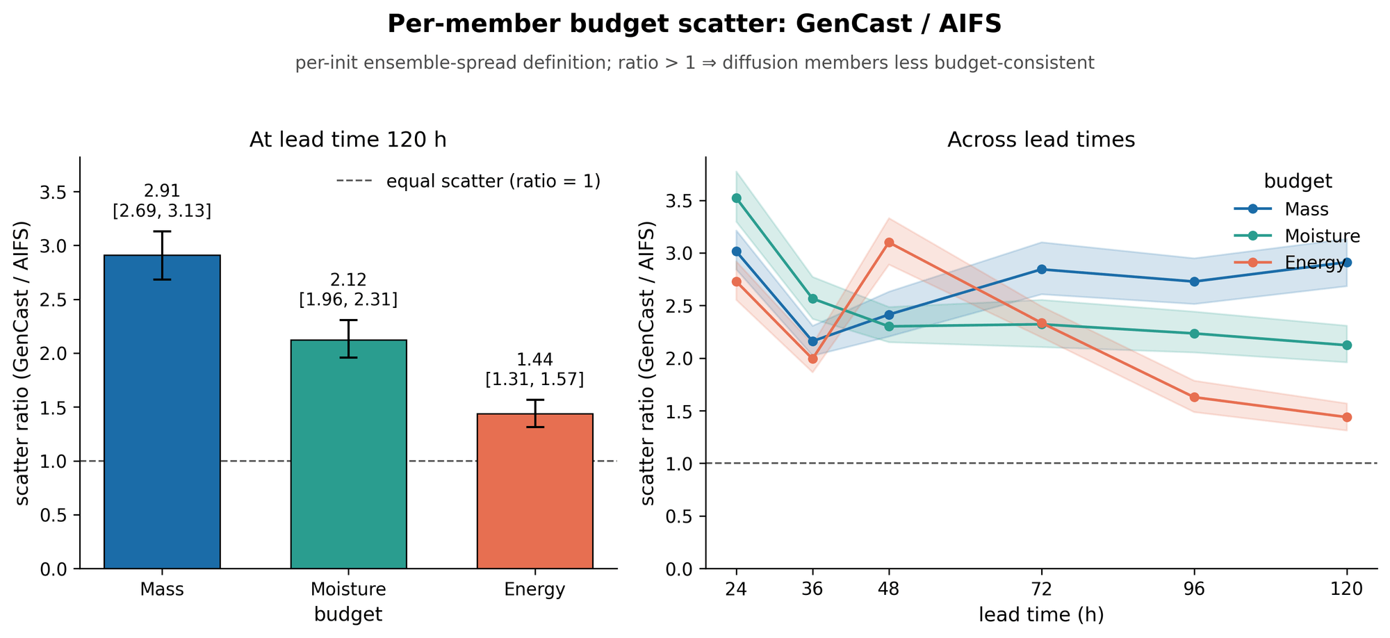
Diffusion conserves on average but not per member, carrying markedly more budget scatter than AIFS across mass, moisture, and energy (2.9× [2.69, 3.13] per-member scatter). A model can therefore have the right marginal tail and still be physically incoherent draw by draw, which matters the moment a single ensemble member is used to drive a downstream hydrological or power-system model rather than being averaged away.

The ranking flips with the book

The sharpest lesson is that a single “which model is better” number does not survive contact with a decision. On a pre-registered day-ahead wind-power backtest over 66 paired delivery days, two operational-grade AI ensembles that agree on the marginal extreme tail part ways the moment the forecast is turned into money. Under one frozen decision rule, the sign of the imbalance-cost difference reverses between the German and the British book (+0.0070 DE / −0.0122 GB (CF)).

The mechanism behind the flip is not mean accuracy. It is where each ensemble’s lower tail sits relative to the commitment quantile the newsvendor problem picks out. Neither ensemble is calibrated there, and the two miss in opposite directions, one over-committing and the other under-committing, so which one costs less depends on the wind regime of the portfolio. Read as a function of the cost-loss ratio rather than at a single operating point, the comparison crosses over (α* = 0.025 [0.018, 0.078]), and the crossover is what a scalar skill score hides. A leaderboard that reports one winner is not wrong so much as under-specified, because it has quietly fixed a decision context the user never agreed to.

There is a matching result on the upside. On the forecast-conditioned Brier skill of record-breaking events, the diffusion ensemble beats the CRPS-trained one by a margin whose permutation test does not close over zero (ΔBSS +0.085, p<10⁻⁴). Sharpness helps when the event is genuinely rare and costs recall when it is not, so even the record-event edge is a trade-off rather than a verdict. It points the same moral as the flip. The right model is the one matched to the loss, read off the decision, and not off a leaderboard.

What an honest tail evaluation looks like

The point of pre-registration is that it makes the flip load-bearing. When the hypotheses, the decision rules, and every amendment are dated and frozen before any season data is read, the reversal cannot be a garden-of-forking-paths artefact discovered by trying portfolios until one obliged. The same discipline forces the nulls into the open. On a four-city temperature book the two models are statistically indistinguishable, and a spatial tail-dependence ordering that looks clean in the point estimates does not survive the date bootstrap. Those are reported as results, because an evaluation that only ever finds effects is telling you more about its own degrees of freedom than about the models.

So the honest answer is not that AI weather models miss the extremes, full stop, nor that they secretly handle them fine. They miss, for a reason written into the loss they are trained on, and the miss is organised, measurable, and often no worse than the physics ensemble it is compared against. What decides whether the miss matters is not the model. It is the decision standing behind the forecast, and whether anyone has bothered to evaluate the tail on that decision’s own terms.