Case study
Cascade
Weather-shock propagation across the European energy graph.
- Weather-shock propagation
- Graph learning
- Language conditioning
- Predictability limits
- Cascade infrastructure graph357 nodes / 675 edges
- Cascade stress-ranking AUC0.738 vs 0.652 persistence
- Cascade onset classifier (negative result)AUC 0.35 vs 0.65 pre-registered bar
The problem
Weather shocks do not stay where they land. A cold, near-windless week over Germany raises gas burn, tightens interconnector flows across the continent, and surfaces days later as a price spike in Italy and a curtailment notice at an aluminium smelter. Cascade models that propagation explicitly. The energy system becomes a typed graph (357 nodes / 675 edges), every coupling between its parts carries a physical mechanism written in language, and a learned operator advances stress along the edges from six hours to fourteen days ahead. The framework is general, and this repository instantiates it end to end for the European energy system across ten years of hourly data and a curated catalogue of shock episodes (59 curated shock episodes), from Storm Niklas to the 2022 gas crisis to the Dunkelflauten of 2024.
One coupled network
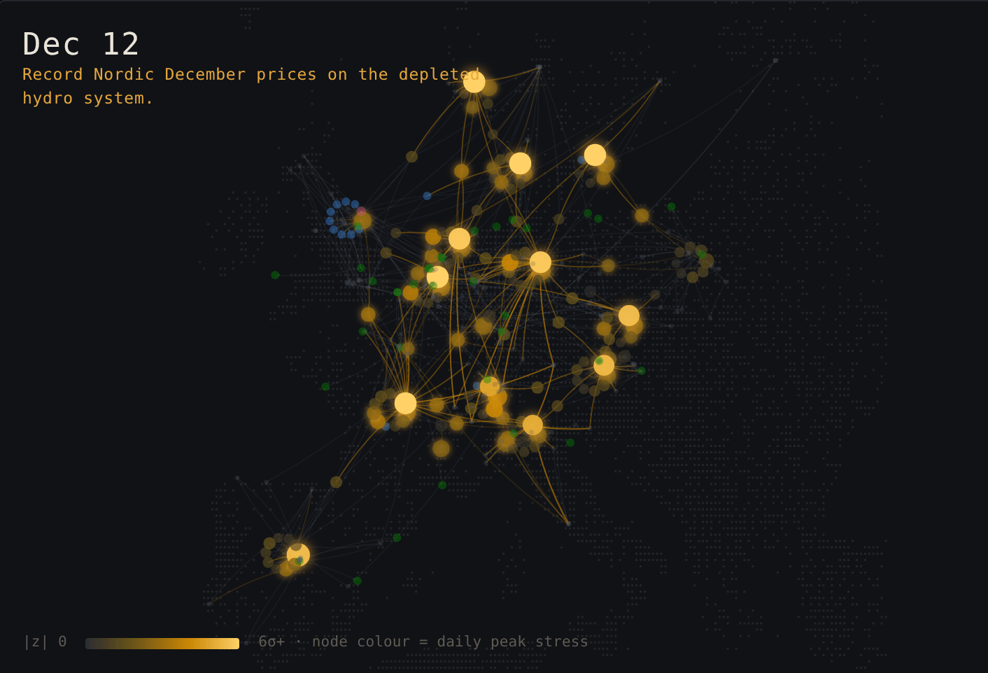
The same coupling Cascade models at continental scale: a weather shock propagating through the energy system to losses. Hover a node, or focus one from the list, to trace its downstream effects.
Approach
The distinctive move is to put language on the edges. Every edge carries a short description of its causal mechanism (direction, channel, timescale), generated by an LLM under typed, quality-gated prompt templates and embedded with a sentence encoder, and the operator conditions its message passing on that text. A matched-capacity ablation then measures exactly what the language buys.
Evaluation is event-sliced, not average-day. Models are judged inside the curated shock episodes (storms, heatwaves, droughts, supply crises, Dunkelflauten), with splits by calendar year and guard bands to stop leakage, a rare-positive onset metric pooled over within-episode pairs with cluster-bootstrap confidence intervals, and a headline experiment scored against a pre-registered success bar. Judging a propagation model on ordinary weather days would flatter it precisely where it matters least.
Results
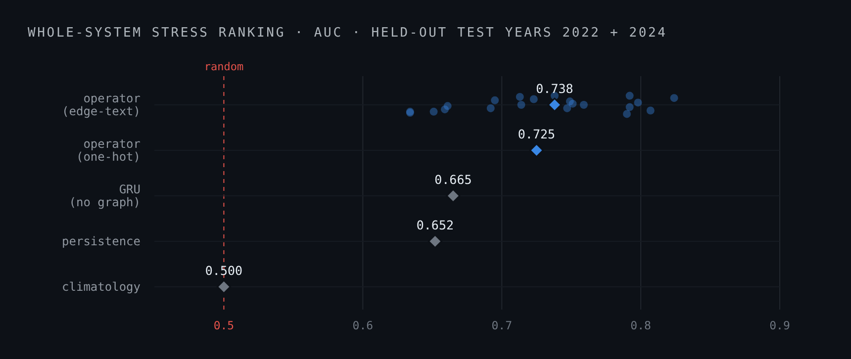
On the held-out test years (2022 and 2024, spanning the gas crisis and the storm winter), the operator ranks stressed against quiet nodes well above persistence (0.738 vs 0.652 persistence). It clears persistence on the large majority of the test episodes it never trained on, and removing the graph forfeits roughly half the margin, so the propagation structure is doing real work rather than decorating a per-node baseline.
The result the deep dive defends hardest is a negative one. Onset of disruption at previously quiet nodes is not recoverable from node history on this graph (AUC 0.35 vs 0.65 pre-registered bar), and it fails three independent ways: the quantile median, an upper-tail rule, and a purpose-built class-weighted exceedance classifier all land below the bar. The shared failure mode is structural, not a tuning miss. Quietness predicts staying quiet, so every history-conditioned score sorts the eventual spikers to the bottom, and the graph-neighbour signal is too faint to override a node’s own autocorrelation. Knowing where that boundary of predictability sits is the deliverable a risk carrier actually needs, and it is worth more than an inflated headline that hides it.
Two further findings sharpen the picture. The operator reads the edge language but gains no in-distribution skill from it: shuffling the mechanism text moves outputs substantially, yet the text arm only ties its one-hot control where it counts, and on held-out edge types the specific semantics turn into specific brittleness. And the forecaster is over-confident in its tails, its central band covering well short of nominal (66% vs 80% nominal), the under-dispersion of a variance-shrinking objective and the same mechanism behind the onset failure.
> ENGINE_ROOM The operator, the pinball objective, and why onset fails
Each node encodes its recent history (a fixed window of hourly z-anomalies) with a GRU together with a node-type embedding. Rounds of message passing then propagate state along the graph, with every message conditioned on its edge’s feature vector: the projected text embedding in the language arm, or a type one-hot in the matched control. A quantile head emits P10, P50, and P90 at each horizon, trained with an anomaly-weighted pinball loss
which penalises the -quantile asymmetrically so that, minimised, recovers the conditional -quantile. That same objective is the root of both the onset failure and the tail over-confidence: a variance-shrinking loss pulls the quantiles inward, so the model under-disperses, and a node with no history of stress is scored as the least likely to light up next. The boundary of predictability is therefore not a data-volume problem to be trained away but a structural property of conditioning on a node’s own quiet past.
The system definition is plain YAML throughout (zones, weather regions, interconnectors, generation fleets, gas infrastructure, industries, and the shock catalogue), ingested from open reanalysis, river-discharge, and market-transparency sources into z-anomalies against an hour-of-year climatology. Every pipeline stage is resumable, and the built graph, mechanism text included, ships with the repository so the operator and its evaluation run out of the box.
What this demonstrates
Weather-to-price propagation modelled across the continental energy system, with a stress ranking that beats persistence on unseen crisis episodes. The graph earns its place: removing it forfeits roughly half the margin.
A measured boundary of predictability. Establishing where onset is and is not forecastable, and defending the negative three independent ways, is exactly the question a risk carrier must answer before pricing propagation risk.
Language-conditioned graph learning with an honest ablation: the model reads the edge text yet gains no in-distribution skill from it, and the calibration and onset failures trace to a single, named property of the training objective.